Peer-to-Peer (p2p) lending industry is causing significant disruption in the loan industry by giving power to individuals and retailers to fund loans, hence, shifting the focus away from the traditional institutions such as banks and non-banking financial corporations (NBFCs).  Borrowers can get loans from retailers at reduced costs resulting in more money pouring into the financial mainstream.  The current article aims at enhancing the investor’s understanding of how the underlying financial instrument, viz., loans, function in the P2P Lending business.  The article explores the parameters that affect Return on Investment of a portfolio of loans.  A better understanding of such parameters will allow the investors to make decisions based on individual’s risk appetite.  Faircent has developed a tool called Portfolio What-if Analysis (PWA) that was used to conduct the current research.

Background

An individual lender can give loans to multiple borrowers, thereby, building a loan portfolio for the self.  In other words, a loan can get funded by multiple lenders and a lender can partially fund multiple loans.  There is a many-to-many relationship between loans and lenders.  A loan is characterized by multiple attributes such as duration, the rate of interest (ROI), amount, start date and purpose.  This article focuses on the impact of these parameters on the return on investment of a portfolio as measured by Net Annualized Return (NAR).  NAR represents the rupee average monthly return of a portfolio measured at annualized level (monthly return is compounded to annual level).  Additionally, principal returned and interest earned along with loss accrued are plotted over time.  Further details on NAR calculations can be found at NAR explanation page.

The current study also explores the impact of loan default.  A loan is considered to have defaulted (resulting in a loss) if any of its Estimated Monthly Instalment (EMI) payment is not paid for more than 180 days.  It is also assumed that if any EMI defaults then all the remaining EMIs will also default.  The principal of these unpaid EMIs is treated as the loss.

The research presented in this article has been conducted using the Portfolio What-if Analysis (PWA) tool developed by Faircent.com.  This online tool can be accessed from Portfolio What-if Analysis . The tool can be accessed from the Lender Dashboard also and a registered lender can save the simulation work.

Single Loan and Multi-Loan Portfolios

Let us build a single loan portfolio with a principal investment of Rs. 1,00,000; duration of 24 months; and ROI of 20%.  NAR, profit (interest earned) and principal returned are shown as a function of time in Figure 1.  The figure shows that the rate at which interest is earned is steep initially.  At the end of the loan period, it plateaus out.  Principal recovery is an almost straight line.  NAR is seen flat at slightly less than 22% for the entire loan period.  If EMIs are paid regularly and there is no loan default then the NAR of a single loan portfolio does not change.

 

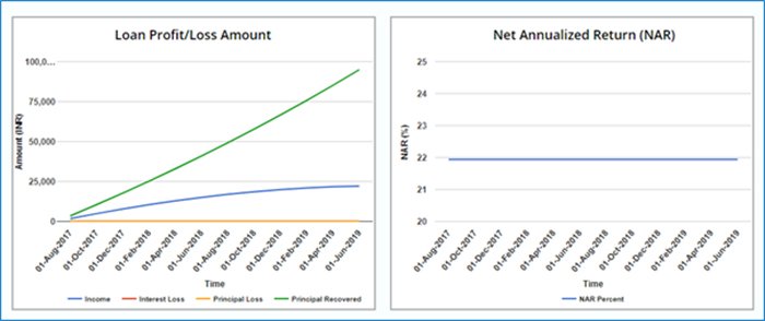
Figure 1: Principal, income, and NAR realized w.r.t. time for a single loan portfolio.

 

If the loan defaults at any stage (any EMI not paid for more than 180 days), the NAR of the portfolio drops steeply.  Figure 2 shows that NAR at the end of the loan duration is 6%, down from 22% with the curve continuously pointing downwards.  This suggests that a single loan portfolio is a risky one with limited chances of recovery.  There can be heavy losses in the investment depending on when the default occurs.  Investments, therefore, should be diversified.

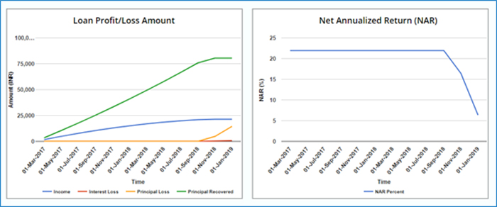
Figure 2: Impact of default on returns for a single loan portfolio

 

An avid investor will also realize that the NAR of a non-defaulting portfolio is primarily dependent on the ROI of the loans.  If a portfolio has multiple loans with different tenures, start dates and amounts but the same ROI then the NAR remains unchanged.  Figure 3 shows the NAR of a portfolio with an initial investment amount of Rs 1,00,000 but divided into loans of varying amounts and tenures.  It is interesting to note that the curve for principal returned is sigmoidal and not as steep as that for a single loan (see Fig 3).

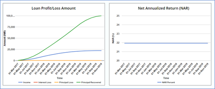
Figure 3: Returns of a multi-loan portfolio

 

What if a couple of loans in the multi-loan portfolio default?  Figure 4 represents a scenario where two out of ten loans default.  There are still eight loans that are not defaulting!  Due to the default, the NAR of the portfolio drops but not at a steep rate.  NAR decreases to around 16% and not 6% as was the case of a single loan portfolio.  This is because the interest earned from non-defaulting loans compensates for the losses.  Risk can be diversified by investing in multiple loans.

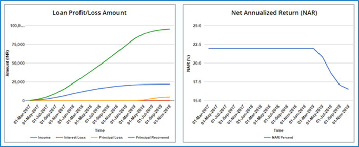
Figure 4: Returns of a defaulting multi-loan portfolio

 

Effect of Various Parameters on Portfolio Return

In this section, we will study the impact of various parameters such as ROI, duration, amount and start date on NAR, principal realized and interest earned over a period.  A portfolio of three (3) loans was created as shown below in Table 1.

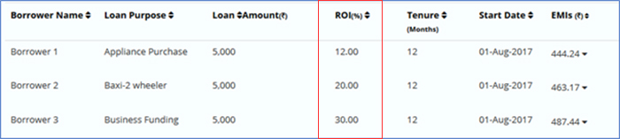
Table 1:  Structure of a multi-loan portfolio with varying ROI but same loan amount, tenure and start date

 

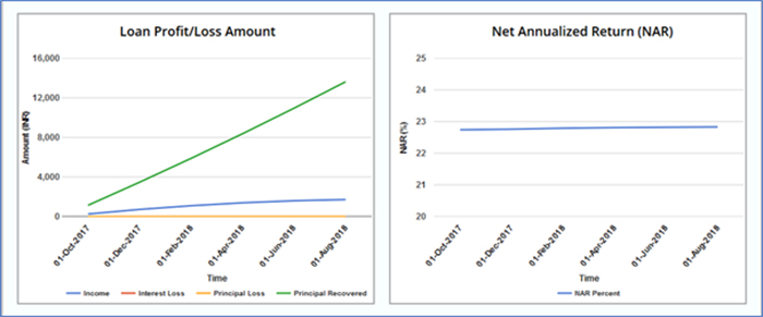
Figure 5: Returns of a multi-loan portfolio with varying ROI.

 

If the amount, tenure and start date remain the same, any change in ROI does not significantly change the variation in NAR over the tenure of the portfolio.  Figure 5 shows that NAR remains almost a constant horizontal line over a period of tenure of the portfolio.  The entire portfolio acts as like a single loan of Rs. 15,000 with a constant EMI over a period of 12 months.

What if we vary the tenure of the loans?  The modified portfolio now has three loans of tenures from 12 to 24 months as shown in Table 2.

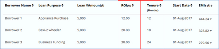
Table 2: Structure of a multi-loan portfolio with varying ROI and tenure but same loan amount and start dates.  The loan with lowest ROI has the shortest tenure.

 

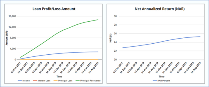
Figure 6:  Returns of a multi-loan portfolio with varying ROI and tenure but same loan amount and start dates.

 

Figure 6 shows that the NAR of the modified portfolio increases over time and the return of the portfolio at the end of 24 months is 25.3%.  NAR is higher than the previous scenario (Fig. 5) by almost 2.5%.  Why is this so?  Over time, the low ROI loan (12%) is exhausted first resulting in a reduced amount of principal outstanding at the end of 12 months.  However, the ROI on the remaining two loans is higher than the one that got exhausted.  This leads to an increase in average monthly returns and the overall NAR of the portfolio over time.  A reverse trend would be witnessed if the low ROI loan has a longer duration (Table 3 and Fig 7).

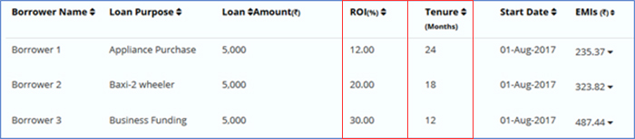
Table 3: Structure of a multi-loan portfolio with varying ROI and tenure but same loan amount and start dates.  The loan with lowest ROI has the longest tenure.

 

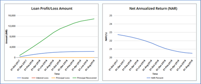
Figure 7: Returns of a multi-loan portfolio with varying ROI and tenure but same loan amount and start dates.  The loan with lowest ROI has the longest tenure.

 

What if we keep loan tenure fixed at 12 months but change the start date of the loans in such a way that the loans are six months apart and the duration of the portfolio is 24 months.  The structure of the modified portfolio is given in Table 4 and the resulting variation of NAR over time in Figure 8.

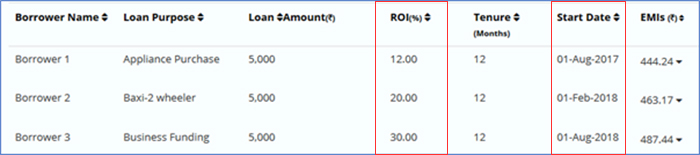
Table 4: Structure of a multi-loan portfolio with varying ROI and different start dates but same tenure and loan amounts.

 

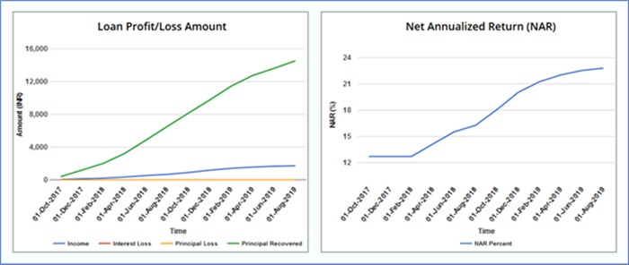
Figure 8: Returns of a multi-loan portfolio with varying ROI and different start dates but same tenure and loan amounts.  The loan with lowest ROI has the earliest start date.

 

Figure 8 shows that NAR of the portfolio increases over time but an increase is not continuous.  For the initial six months, NAR is at 12.7% after which it jumps to 14% and finally ends at 22.8%.  The portfolio NAR initiates with the low ROI loan first and as higher ROI loans are added to the portfolio, the NAR continuously increases with an increase in average monthly returns.

A trend is reversed if the higher ROI loan is added to the portfolio first and lowest RI loan last.  Interestingly, the ending NAR of the portfolio remains the same at 22.8% (see Table 5 and Fig 9).

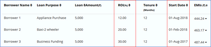
Table 5: Structure of a multi-loan portfolio with varying ROI and different start dates but same tenure and loan amounts. The loan with highest ROI has the earliest start date.

 

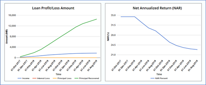
Figure 9: Returns of a multi-loan portfolio with varying ROI and different start dates but same tenure and loan amounts.  The loan with highest ROI has the earliest start date.

 

What if analysis shows that the changes in NAR over time are seen if the portfolio has loans with varying ROI.  NAR remains flat if the portfolio has all loans of the same ROI even if the start date, tenure, and amounts differ.  However, the rate at which income is earned and the principal is returned is strongly dependent on variations in the loan amount, tenure and start date.  The only other time NAR variation is seen for constant ROI loans is when the loans default.  Table 6 and Figure 10 show that all three loans are at 20% ROI, the first loan has defaulted and the NAR drops rapidly from 22%.  However, other loans in the portfolio lead to the recovery of NAR and the total portfolio NAR ends at 7%.

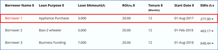
Table 6:  Structure of a multi-loan with the different loan amount and start dates but same ROI and tenure.  The loan with the lowest loan amount is considered to have defaulted.

 

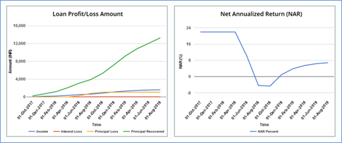
Figure 10: Returns of a multi-loan portfolio with different loan amounts and start dates but same ROI and tenure.  The loan with the lowest loan amount is considered to have defaulted.

 

Summary

This study explores the impact of loan parameters on portfolio returns.  The returns are studied in terms of Net Annualized Return, recovery of principal, interest earned and losses accumulated.  It is seen that the loan interest rate (ROI) has a significant impact on NAR and its variation over time.  Portfolio with constant ROI does not impact the portfolio’s NAR unless there is a default.  Tenure, start date and loan amount have an impact on the rate at which the principal is recovered and income is generated but does not impact NAR variation over time.

A single loan portfolio is a lot riskier than a multi-loan portfolio.  A default of some loans in a multi-loan portfolio can be compensated by income generated by non-defaulting loans.  There is no such option in a single loan portfolio.  Investing smaller amounts in multiple loans is a good risk mitigation strategy.  Investing in newer loans around the time a loan default can lead to the good recovery of portfolio NAR.  Continuous re-investment of loan proceeds and new investments minimizes the impact of defaulting loans and stabilizes the portfolio NAR.